Figure 1: Shown at top right is the output of a 5V switch-mode power supply acquired with an RP4030 active voltage-rail probe

Performing a fast Fourier transfer (FFT) on an oscilloscope can be likened to driving a car. Just as there are two dominant strains of power-train transmissions, there are two dominant approaches to transferring signals acquired on an oscilloscope from the time domain to the frequency domain. There's the stickshift approach, in which the FFT parameters are set manually, and the automatic approach, in which you let the oscilloscope make decisions for you.

Now let's look at a real-world example of an FFT acquisitions. First, we'll acquire the output signal from a simple 5-V switch-mode power supply using a Teledyne LeCroy RP4030 active voltage-rail probe (Figure 1). The power supply is drawing about 100 mA. The WavePro HD oscilloscope is set for 200 mV/division, and the acquisition reveals some switching noise as well as other noise. The horizontal timebase is at 1 ms/division. We can surmise that there are perhaps two or three cycles per millisecond, which extrapolates to a switching frequency of about 3-4 kHz for the power supply. Thus, we will be looking at low-frequency noise.
 

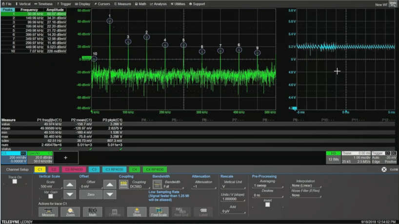
Figure 2: At top center is the frequency-domain plot of the power supply's output waveform with averaging.

Next, we'll apply our oscilloscope's spectral analysis Math function to the power supply's output waveform, which is on Channel 3 of our instrument (Figure 2). Most of the noise is in the low-frequency range, but not all. We're looking at averaging of 10 spectrum cycles here. Applying averaging to the spectral analysis makes it easier to read and digest.

We noted that, as expected, most of the noise was at low frequencies, but we'd like to get a better look at what's happening at higher frequencies. Figure 2 only spans up to 500 kHz, so we'll tell our spectral analysis function to look at a frequency range of up to 10 MHz. That will automatically tell the oscilloscope to increase the sampling rate from 2.5 MS/s to 50 MS/s. The resolution stays the same, so our timebase remains at 1 ms/division, giving us 500 kS of data.
 

Figure 3: Opening up the top frequency to 10 MHz reveals a large amount of noise in the 2-3 MHz range

With our highest frequency at 10 MHz, we can see that there's quite a bit of noise in the 2-3 MHz range, and many harmonics of the noise out to our frequency limit (Figure 3). Bearing in mind our vertical scale of 200 mV/division, we might want to increase the gain because we're not using the full-scale resolution. It likely won't change the noise much but if you have headroom, it's a good idea to take advantage of it. Figure 3 shows that the noise varies to some degree; there's some periodicity to our little switch-mode power supply.

Next, we can change the upper limit of our FFT to 1 GHz while also decreasing the resolution so as not to have quite so many data points. What we find is that most of the noise is in the range of 100 MHz and below. Additionally, that noise peaks out at about -30 dBmV, or about 30 µV, which is a rather trivial amount.
 

Figure 4: A final 100-MHz-wide look at our 5-V power supply output shows a 1-mV peak at about 16 MHz

So we'll once again narrow down our FFT frequency range to 100 MHz for a last
look (Figure 4). Bear in mind, again, that this is 30 µV of noise on a 5-V rail. Other than the preponderance of noise in the 2-3 MHz, range, the largest peak, at about 16 MHz, is roughly at a 1-mV level. A number of spurious peaks appear at higher frequencies as well.

Note that we can control the spectrum analyzer by manipulating the highest frequency in the spectrum and the resolution. Those parameters, in turn, automatically control the oscilloscope's horizontal timebase and acquisition rate. But from our example, it's clear that looking at a signal in the frequency domain gives us a great deal of information about it that we simply cannot get from the time-domain view.